Practice: Seismic Data and Fourier Analysis - EPS 164 Seismology Course Materials

Colab note: This notebook is designed to run on Google Colab. The first code cell installs dependencies.

Learning Objectives:

Understand the Fourier transform as a decomposition into sinusoids
Relate time-domain signals to their frequency-domain representations
Understand the effects of integration and differentiation on signals and their spectra
Download and process real seismic data
Apply Fourier analysis to understand seismic wave spectral content
Remove instrument response from seismic data

Prerequisites: Basic Python, trigonometry, calculus

Reference: Shearer, Chapter 11 - Seismometers and Seismographs

Notebook Outline: Notebook Outline:

1. Theory - Fourier Analysis with Toy Problems
2. Real Observations - Seismic Data Analysis
Summary: Theory Meets Observation
- Next Steps

This notebook introduces two fundamental concepts in seismology:

Signal processing: How we analyze seismic waveforms using Fourier analysis

# Install dependencies (for Google Colab or missing packages)
import sys

# Check if running in Colab
try:
    import google.colab
    IN_COLAB = True
    print("Running in Google Colab")
except:
    IN_COLAB = False
    print("Running in local environment")

# Install required packages if needed
required_packages = {
    'numpy': 'numpy',
    'matplotlib': 'matplotlib',
    'scipy': 'scipy',
    'obspy': 'obspy'
}

missing_packages = []
for package, pip_name in required_packages.items():
    try:
        __import__(package)
        print(f"✓ {package} is already installed")
    except ImportError:
        missing_packages.append(pip_name)
        print(f"✗ {package} not found")

if missing_packages:
    print(f"\nInstalling missing packages: {', '.join(missing_packages)}")
    import subprocess
    subprocess.check_call([sys.executable, "-m", "pip", "install", "-q"] + missing_packages)
    print("✓ Installation complete!")
else:
    print("\n✓ All required packages are installed!")

Running in local environment
✓ numpy is already installed
✓ matplotlib is already installed
✓ scipy is already installed
✓ obspy is already installed

✓ All required packages are installed!

# Import libraries
import numpy as np
import matplotlib.pyplot as plt
from scipy.fft import fft, fftfreq, ifft
from scipy.signal import butter, filtfilt
from scipy.integrate import cumulative_trapezoid
import warnings
warnings.filterwarnings('ignore')

plt.style.use('default')

# Set plotting defaults
plt.rcParams['figure.figsize'] = (12, 6)
plt.rcParams['font.size'] = 11

print("Libraries loaded successfully!")

Libraries loaded successfully!

1. Theory - Fourier Analysis with Toy Problems¶

1.1 What is a Fourier Transform?¶

The Fourier Transform is a mathematical operation that decomposes a signal into its constituent frequencies. It’s based on the fundamental idea that any signal can be represented as a sum of sinusoids (sines and cosines) with different:

Frequencies (how fast they oscillate)
Amplitudes (how strong they are)
Phases (where they start)

Key Insight: A signal can be viewed in two equivalent ways:

Time Domain: Amplitude vs. time → what we measure
Frequency Domain: Amplitude vs. frequency → what frequencies are present

Mathematical Definition:

For a continuous signal $x(t)$ :

X(f) = \int_{-\infty}^{\infty} x(t) e^{-2\pi i f t} dt

(1)

For a discrete signal $x[n]$ (what we have in computers):

X[k] = \sum_{n=0}^{N-1} x[n] e^{-2\pi i k n / N}

(2)

where:

$X(f)$ or $X[k]$ is the Fourier transform (complex-valued)
$f$ is frequency in Hz
$i = \sqrt{-1}$

Don’t worry about the complex exponentials - we’ll build intuition with simple examples!

1.2 Toy Problem 1: A Single Sinusoid¶

Let’s start with the simplest possible signal: a pure sine wave.

x(t) = A \sin(2\pi f_0 t)

(3)

where:

$A$ = amplitude
$f_0$ = frequency in Hz (cycles per second)
$t$ = time in seconds

Question: What will the Fourier transform look like?

# Create a single sine wave
duration = 2.0  # seconds
sampling_rate = 100  # Hz (samples per second)
t = np.arange(0, duration, 1/sampling_rate)

# Signal parameters
A = 1.0  # amplitude
f0 = 5.0  # frequency in Hz

# Generate signal
x = A * np.sin(2 * np.pi * f0 * t)

# Compute Fourier Transform
N = len(x)
X = fft(x)
freqs = fftfreq(N, 1/sampling_rate)

# Only plot positive frequencies (FFT is symmetric for real signals)
positive_freqs = freqs[:N//2]
X_magnitude = np.abs(X[:N//2]) * 2/N  # Normalize

# Plot
fig, (ax1, ax2) = plt.subplots(2, 1, figsize=(12, 8))

# Time domain
ax1.plot(t, x, 'b-', linewidth=1.5)
ax1.set_xlabel('Time (s)', fontsize=12)
ax1.set_ylabel('Amplitude', fontsize=12)
ax1.set_title(f'Time Domain: Pure Sine Wave (f = {f0} Hz)', fontsize=13, fontweight='bold')
ax1.grid(True, alpha=0.3)
ax1.set_xlim([0, 1])  # Show first second

# Frequency domain
ax2.stem(positive_freqs, X_magnitude, basefmt=' ', linefmt='r-', markerfmt='ro')
ax2.set_xlabel('Frequency (Hz)', fontsize=12)
ax2.set_ylabel('Amplitude', fontsize=12)
ax2.set_title('Frequency Domain: Fourier Transform', fontsize=13, fontweight='bold')
ax2.grid(True, alpha=0.3)
ax2.set_xlim([0, 20])

plt.tight_layout()
plt.show()

print(f"Signal: {A} * sin(2π * {f0} * t)")
print(f"Fourier Transform: Single peak at f = {f0} Hz")
print("\nKey Observation: A pure sine wave contains ONLY ONE frequency!")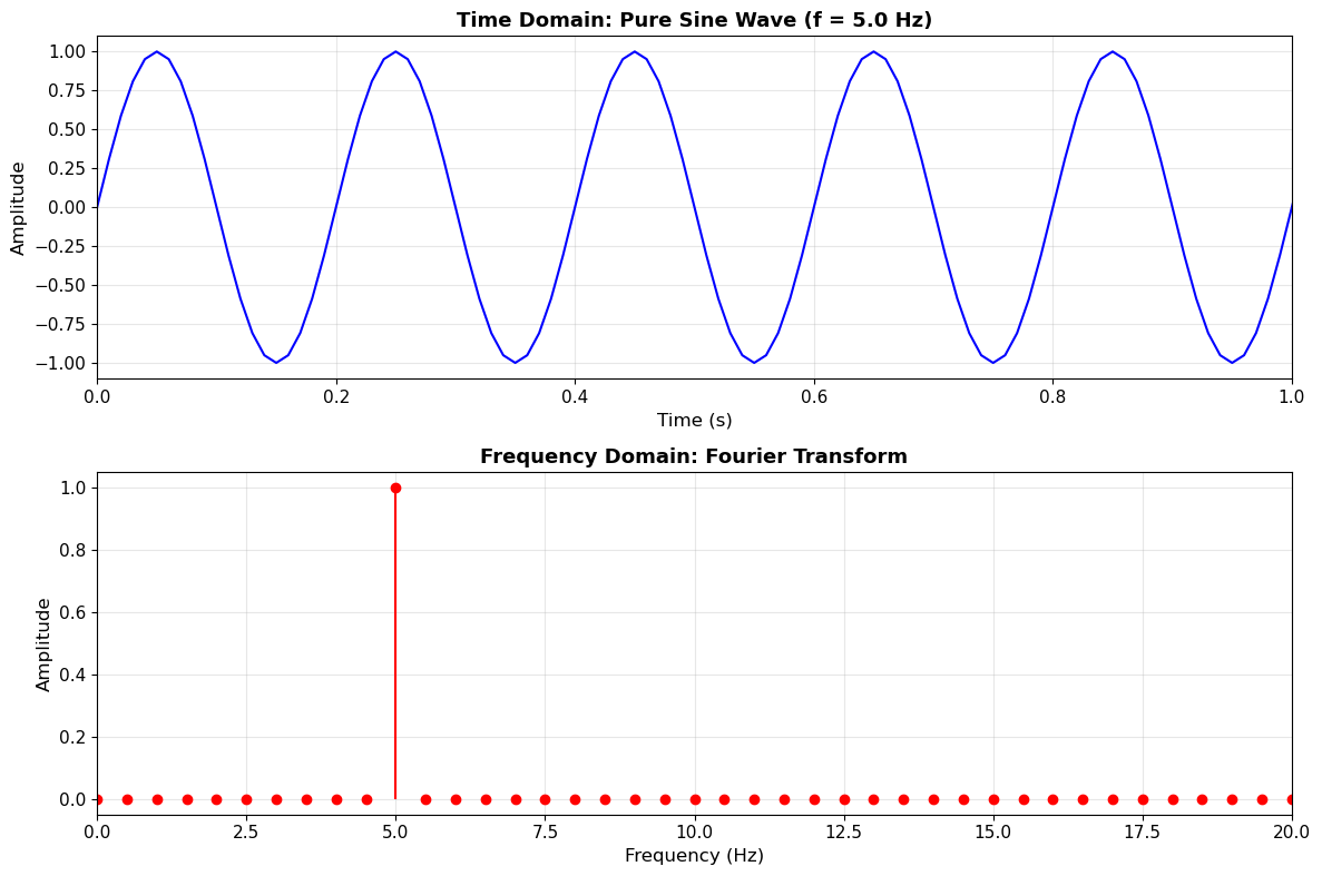

Signal: 1.0 * sin(2π * 5.0 * t)
Fourier Transform: Single peak at f = 5.0 Hz

Key Observation: A pure sine wave contains ONLY ONE frequency!

1.3 Toy Problem 2: Sum of Multiple Sinusoids¶

Real signals (like seismic waves) contain multiple frequencies. Let’s add three sine waves together:

x(t) = A_1 \sin(2\pi f_1 t) + A_2 \sin(2\pi f_2 t) + A_3 \sin(2\pi f_3 t)

(4)

Question: What will the Fourier transform show?

# Create a signal with three frequencies
f1, f2, f3 = 2, 5, 10  # Hz
A1, A2, A3 = 1.0, 0.7, 0.4  # Amplitudes

# Generate composite signal
x_multi = A1 * np.sin(2*np.pi*f1*t) + A2 * np.sin(2*np.pi*f2*t) + A3 * np.sin(2*np.pi*f3*t)

# Compute Fourier Transform
X_multi = fft(x_multi)
X_multi_magnitude = np.abs(X_multi[:N//2]) * 2/N

# Plot
fig, (ax1, ax2) = plt.subplots(2, 1, figsize=(12, 8))

# Time domain
ax1.plot(t, x_multi, 'b-', linewidth=1.5, label='Composite signal')
ax1.plot(t, A1*np.sin(2*np.pi*f1*t), 'r--', alpha=0.5, linewidth=1, label=f'{f1} Hz component')
ax1.plot(t, A2*np.sin(2*np.pi*f2*t), 'g--', alpha=0.5, linewidth=1, label=f'{f2} Hz component')
ax1.plot(t, A3*np.sin(2*np.pi*f3*t), 'm--', alpha=0.5, linewidth=1, label=f'{f3} Hz component')
ax1.set_xlabel('Time (s)', fontsize=12)
ax1.set_ylabel('Amplitude', fontsize=12)
ax1.set_title('Time Domain: Sum of Three Sine Waves', fontsize=13, fontweight='bold')
ax1.legend(loc='upper right')
ax1.grid(True, alpha=0.3)
ax1.set_xlim([0, 2])

# Frequency domain
ax2.stem(positive_freqs, X_multi_magnitude, basefmt=' ', linefmt='r-', markerfmt='ro')
ax2.axvline(f1, color='red', linestyle=':', alpha=0.5, label=f'{f1} Hz')
ax2.axvline(f2, color='green', linestyle=':', alpha=0.5, label=f'{f2} Hz')
ax2.axvline(f3, color='magenta', linestyle=':', alpha=0.5, label=f'{f3} Hz')
ax2.set_xlabel('Frequency (Hz)', fontsize=12)
ax2.set_ylabel('Amplitude', fontsize=12)
ax2.set_title('Frequency Domain: Fourier Transform Shows All Three Frequencies', fontsize=13, fontweight='bold')
ax2.legend()
ax2.grid(True, alpha=0.3)
ax2.set_xlim([0, 15])

plt.tight_layout()
plt.show()

print(f"Signal components: {A1}*sin(2π*{f1}*t) + {A2}*sin(2π*{f2}*t) + {A3}*sin(2π*{f3}*t)")
print(f"Fourier Transform: Three peaks at {f1}, {f2}, and {f3} Hz")
print("\nKey Observation: Fourier transform DECOMPOSES the signal into its constituent frequencies!")
print("The amplitude of each peak tells us how much of that frequency is present.")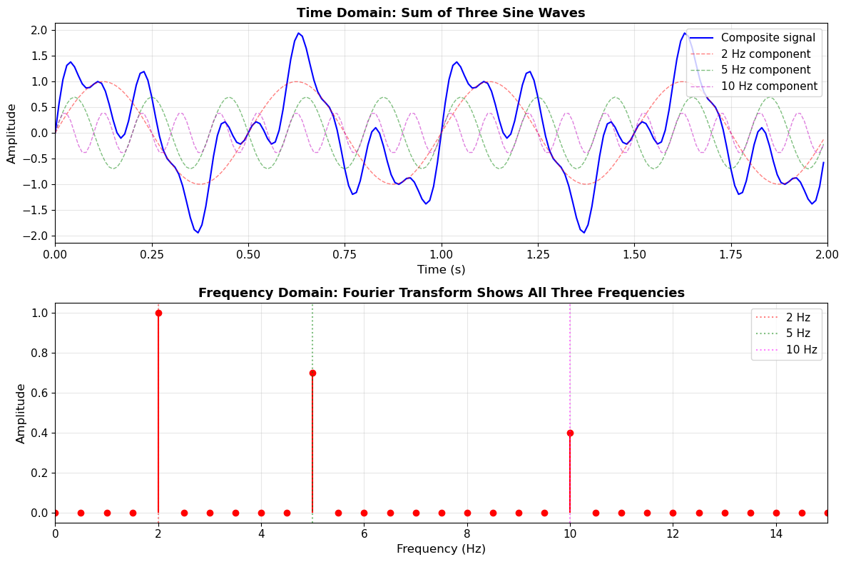

Signal components: 1.0*sin(2π*2*t) + 0.7*sin(2π*5*t) + 0.4*sin(2π*10*t)
Fourier Transform: Three peaks at 2, 5, and 10 Hz

Key Observation: Fourier transform DECOMPOSES the signal into its constituent frequencies!
The amplitude of each peak tells us how much of that frequency is present.

1.4 Integration and Differentiation: Time Domain Effects¶

In seismology, we often need to convert between:

Acceleration → Velocity → Displacement

These are related by integration (or equivalently, differentiation in reverse):

\text{velocity}(t) = \int \text{acceleration}(t) \, dt

(5)

\text{displacement}(t) = \int \text{velocity}(t) \, dt

(6)

Let’s see what integration does to a sinusoid in the time domain:

For $x(t) = A \sin(2\pi f t)$ :

\int x(t) \, dt = -\frac{A}{2\pi f} \cos(2\pi f t) + C

(7)

Key observation:

Integration divides amplitude by $2\pi f$
Low frequencies (small $f$ ) → Large amplitude increase
High frequencies (large $f$ ) → Small amplitude increase

# Demonstrate integration on our multi-frequency signal
dt = 1/sampling_rate

# Start with "acceleration"
acceleration = x_multi.copy()

# Integrate once to get "velocity"
velocity = cumulative_trapezoid(acceleration, dx=dt, initial=0)

# Integrate again to get "displacement"
displacement = cumulative_trapezoid(velocity, dx=dt, initial=0)

# Plot all three
fig, axes = plt.subplots(3, 1, figsize=(14, 10))

# Acceleration
axes[0].plot(t, acceleration, 'b-', linewidth=1.5)
axes[0].set_ylabel('Acceleration\n(arbitrary units)', fontsize=11)
axes[0].set_title('Effect of Integration in Time Domain', fontsize=14, fontweight='bold')
axes[0].grid(True, alpha=0.3)
axes[0].set_xlim([0, 2])

# Velocity
axes[1].plot(t, velocity, 'g-', linewidth=1.5)
axes[1].set_ylabel('Velocity\n(= ∫ acceleration dt)', fontsize=11)
axes[1].grid(True, alpha=0.3)
axes[1].set_xlim([0, 2])

# Displacement
axes[2].plot(t, displacement, 'r-', linewidth=1.5)
axes[2].set_ylabel('Displacement\n(= ∫ velocity dt)', fontsize=11)
axes[2].set_xlabel('Time (s)', fontsize=12)
axes[2].grid(True, alpha=0.3)
axes[2].set_xlim([0, 2])

plt.tight_layout()
plt.show()

print("Notice how integration:")
print("1. Smooths the signal (removes high frequencies)")
print("2. Amplifies low-frequency content")
print("3. Changes the phase (sine ↔ cosine)")
print("\nThis is why seismograms look different when showing acceleration vs. displacement!")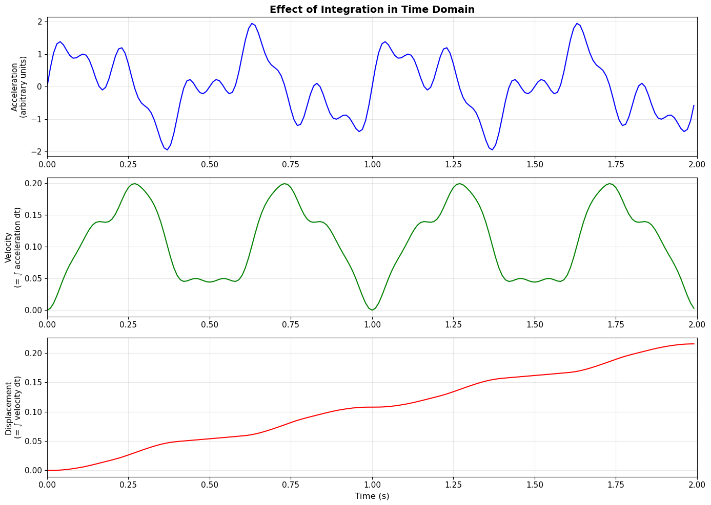

Notice how integration:
1. Smooths the signal (removes high frequencies)
2. Amplifies low-frequency content
3. Changes the phase (sine ↔ cosine)

This is why seismograms look different when showing acceleration vs. displacement!

1.5 Integration and Differentiation: Frequency Domain Effects¶

The same operations look very different in the frequency domain!

Mathematical relationship:

If $x(t) \leftrightarrow X(f)$ (Fourier transform pair), then:

Integration: $\int x(t) dt \leftrightarrow \frac{X(f)}{2\pi i f}$
Differentiation: $\frac{dx}{dt} \leftrightarrow 2\pi i f \cdot X(f)$

Key insight:

Integration → Divide spectrum by $f$ → Suppresses high frequencies
Differentiation → Multiply spectrum by $f$ → Enhances high frequencies

This is why:

Acceleration recordings emphasize high-frequency shaking
Displacement recordings emphasize low-frequency, permanent ground motion

# Compare spectra of acceleration, velocity, and displacement
fig, (ax1, ax2) = plt.subplots(1, 2, figsize=(14, 5))

# Compute FFTs
Acc_fft = np.abs(fft(acceleration)[:N//2]) * 2/N
Vel_fft = np.abs(fft(velocity)[:N//2]) * 2/N
Disp_fft = np.abs(fft(displacement)[:N//2]) * 2/N

# Linear scale
ax1.plot(positive_freqs, Acc_fft, 'b-', linewidth=2, label='Acceleration', alpha=0.7)
ax1.plot(positive_freqs, Vel_fft, 'g-', linewidth=2, label='Velocity', alpha=0.7)
ax1.plot(positive_freqs, Disp_fft, 'r-', linewidth=2, label='Displacement', alpha=0.7)
ax1.set_xlabel('Frequency (Hz)', fontsize=12)
ax1.set_ylabel('Amplitude (linear)', fontsize=12)
ax1.set_title('Frequency Spectra - Linear Scale', fontsize=13, fontweight='bold')
ax1.legend(fontsize=11)
ax1.grid(True, alpha=0.3)
ax1.set_xlim([0, 15])

# Log scale (clearer view)
ax2.semilogy(positive_freqs[1:], Acc_fft[1:], 'b-', linewidth=2, label='Acceleration', alpha=0.7)
ax2.semilogy(positive_freqs[1:], Vel_fft[1:], 'g-', linewidth=2, label='Velocity', alpha=0.7)
ax2.semilogy(positive_freqs[1:], Disp_fft[1:], 'r-', linewidth=2, label='Displacement', alpha=0.7)
ax2.set_xlabel('Frequency (Hz)', fontsize=12)
ax2.set_ylabel('Amplitude (log scale)', fontsize=12)
ax2.set_title('Frequency Spectra - Log Scale', fontsize=13, fontweight='bold')
ax2.legend(fontsize=11)
ax2.grid(True, alpha=0.3)
ax2.set_xlim([0, 15])

plt.tight_layout()
plt.show()

print("Key Observations:")
print("1. At LOW frequencies: Displacement >> Velocity >> Acceleration")
print("2. At HIGH frequencies: Acceleration >> Velocity >> Displacement")
print("3. Each integration reduces amplitude by factor of (2πf)")
print("\nThis is why:")
print("- Strong motion seismometers record ACCELERATION (captures high-freq shaking)")
print("- Broadband seismometers often show VELOCITY or DISPLACEMENT (long-period waves)")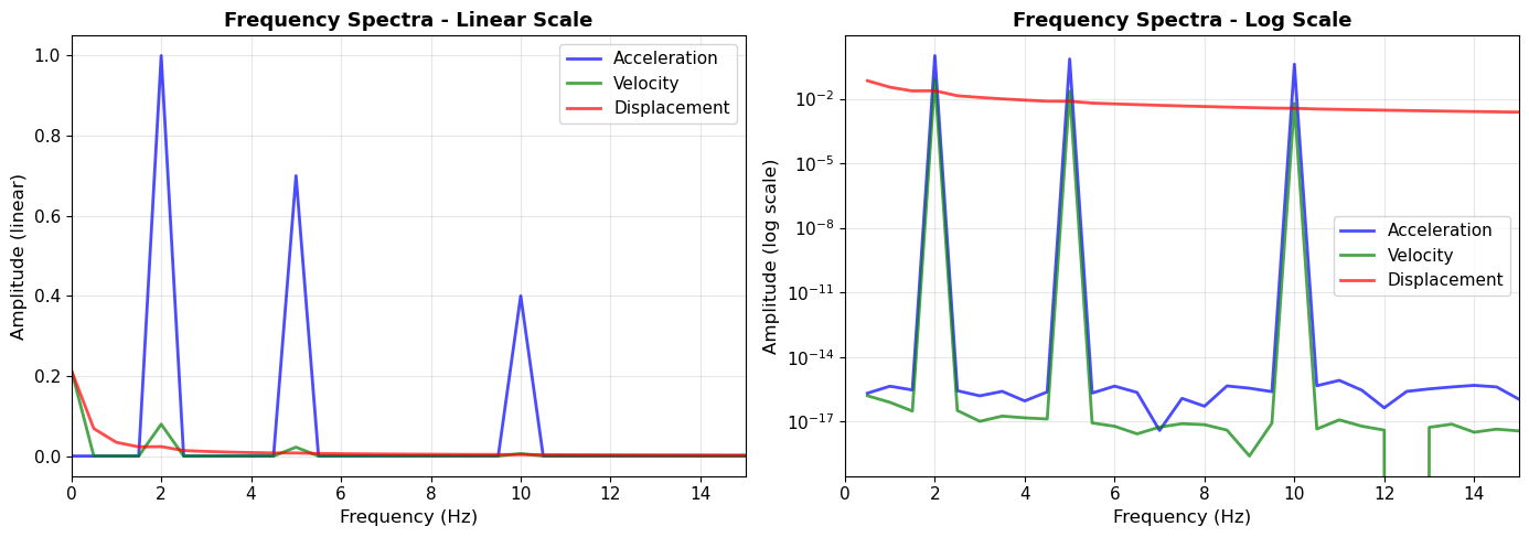

Key Observations:
1. At LOW frequencies: Displacement >> Velocity >> Acceleration
2. At HIGH frequencies: Acceleration >> Velocity >> Displacement
3. Each integration reduces amplitude by factor of (2πf)

This is why:
- Strong motion seismometers record ACCELERATION (captures high-freq shaking)
- Broadband seismometers often show VELOCITY or DISPLACEMENT (long-period waves)

What is a Bandpass Filter?¶

A bandpass filter allows a specific range of frequencies to pass through, while removing frequencies outside that range.

For example, a 4–6 Hz bandpass filter:

keeps signals between 4 and 6 Hz
removes lower-frequency signals (e.g., drift, long-period noise)
removes higher-frequency signals (e.g., high-frequency noise)

In seismology, bandpass filters are often used to:

isolate particular phases
improve signal-to-noise ratio
focus on a frequency band of interest

# Simple bandpass demo
t = np.arange(0, 5, 1/sampling_rate)

x = (np.sin(2*np.pi*1*t) +      # low frequency
     np.sin(2*np.pi*5*t) +      # target
     0.5*np.sin(2*np.pi*12*t))  # high frequency

b, a = butter(4, [4, 6], btype='band', fs=sampling_rate)
x_filt = filtfilt(b, a, x)

plt.figure(figsize=(10,4))
plt.plot(t, x, label='Original')
plt.plot(t, x_filt, label='Filtered (4–6 Hz)')
plt.legend()
plt.title("Bandpass filter isolates the 5 Hz signal")
plt.xlabel("Time (s)")
plt.ylabel("Amplitude")
plt.grid(True, alpha=0.3)
plt.show()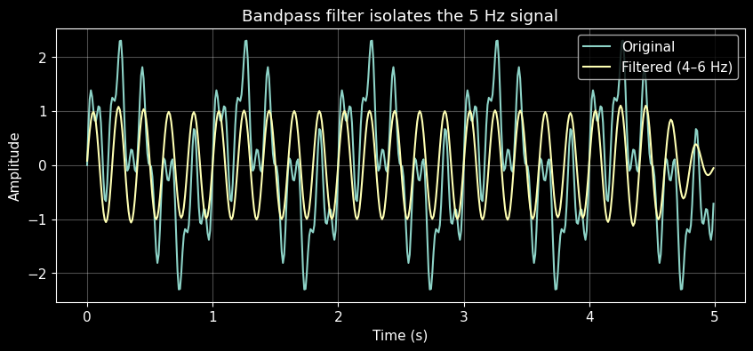

1.6 The Problem: Finite Time Series and Spectral Leakage¶

So far we have been applying Fourier transforms without worrying about what happens at the edges of the time series.

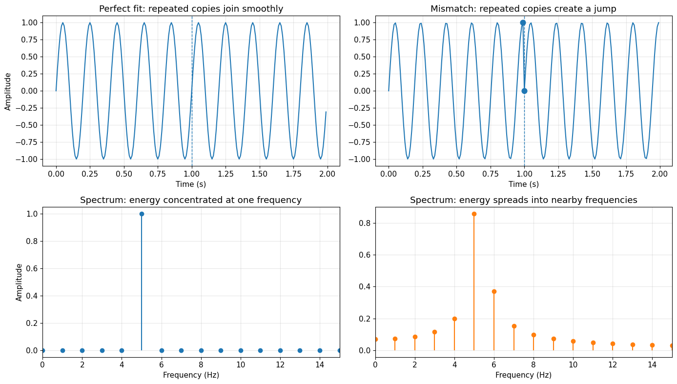
The key issue is that the FFT assumes the signal is periodic: it imagines the finite record repeating forever.

If the signal fits perfectly into the window, this works well. But if it does not fit perfectly, the repeated copies do not join smoothly. The FFT then sees a discontinuity at the boundary, and energy that should be concentrated at one frequency gets spread across nearby frequencies. This is called spectral leakage.

In the next example, we compare two nearly identical signals:

one that fits perfectly in the window
one that does not

The only difference is whether the signal starts and ends consistently when repeated.

# Spectral leakage demo: perfect-fit vs mismatch
duration_leak = 1.0
t_leak = np.arange(0, duration_leak, 1/sampling_rate)

f_fit = 5.0   # exactly 5 cycles in 1 second
f_mis = 5.3   # does not fit the window exactly

x_fit = np.sin(2 * np.pi * f_fit * t_leak)
x_mis = np.sin(2 * np.pi * f_mis * t_leak)

N_leak = len(t_leak)
freqs_leak = fftfreq(N_leak, 1/sampling_rate)[:N_leak//2]

X_fit = fft(x_fit)
X_mis = fft(x_mis)

X_fit_mag = np.abs(X_fit[:N_leak//2]) * 2 / N_leak
X_mis_mag = np.abs(X_mis[:N_leak//2]) * 2 / N_leak

# Show periodic extension explicitly
t_ext = np.concatenate([t_leak, t_leak + duration_leak])
x_fit_ext = np.concatenate([x_fit, x_fit])
x_mis_ext = np.concatenate([x_mis, x_mis])

fig, axes = plt.subplots(2, 2, figsize=(14, 8))

# Perfect fit in time
axes[0, 0].plot(t_ext, x_fit_ext, linewidth=1.5)
axes[0, 0].axvline(duration_leak, linestyle='--', linewidth=1)
axes[0, 0].set_title("Perfect fit: repeated copies join smoothly")
axes[0, 0].set_xlabel("Time (s)")
axes[0, 0].set_ylabel("Amplitude")
axes[0, 0].grid(True, alpha=0.3)

# Mismatch in time
axes[0, 1].plot(t_ext, x_mis_ext, linewidth=1.5)
axes[0, 1].axvline(duration_leak, linestyle='--', linewidth=1)
axes[0, 1].scatter([duration_leak - 1/sampling_rate, duration_leak],
                   [x_mis[-1], x_mis[0]],
                   s=60, zorder=5)
axes[0, 1].set_title("Mismatch: repeated copies create a jump")
axes[0, 1].set_xlabel("Time (s)")
axes[0, 1].grid(True, alpha=0.3)

# Perfect fit spectrum
axes[1, 0].stem(freqs_leak, X_fit_mag, basefmt=" ", linefmt='C0-', markerfmt='C0o')
axes[1, 0].set_xlim(0, 15)
axes[1, 0].set_title("Spectrum: energy concentrated at one frequency")
axes[1, 0].set_xlabel("Frequency (Hz)")
axes[1, 0].set_ylabel("Amplitude")
axes[1, 0].grid(True, alpha=0.3)

# Mismatch spectrum
axes[1, 1].stem(freqs_leak, X_mis_mag, basefmt=" ", linefmt='C1-', markerfmt='C1o')
axes[1, 1].set_xlim(0, 15)
axes[1, 1].set_title("Spectrum: energy spreads into nearby frequencies")
axes[1, 1].set_xlabel("Frequency (Hz)")
axes[1, 1].grid(True, alpha=0.3)

plt.tight_layout()
plt.show()

print("Key observation:")
print("- 5.0 Hz fits perfectly in the 1 second window, so its spectrum is sharp.")
print("- 5.3 Hz does not fit perfectly, so its energy leaks into nearby frequencies.")

Key observation:
- 5.0 Hz fits perfectly in the 1 second window, so its spectrum is sharp.
- 5.3 Hz does not fit perfectly, so its energy leaks into nearby frequencies.

1.7 The Solution: Tapering (Windowing)¶

A taper reduces spectral leakage by gradually bringing the signal toward zero at the edges.

This does not recover lost information. Instead, it reduces the sharp discontinuity that causes the FFT to spread energy across frequencies.

Common tapers include:

Hann
Hamming
Tukey
Cosine tapers

The tradeoff is important:

less leakage
but also slightly broader peaks

So tapering improves spectral cleanliness, but slightly reduces frequency resolution.

# Apply taper to the mismatched signal and compare
from scipy.signal import windows

hann_taper = windows.hann(N_leak)
x_mis_tapered = x_mis * hann_taper

X_mis_tapered = fft(x_mis_tapered)
X_mis_tapered_mag = np.abs(X_mis_tapered[:N_leak//2]) * 2 / N_leak

fig, axes = plt.subplots(2, 2, figsize=(14, 8))

# Original mismatched signal
axes[0, 0].plot(t_leak, x_mis, linewidth=1.5)
axes[0, 0].scatter([t_leak[0], t_leak[-1]], [x_mis[0], x_mis[-1]], s=60, zorder=5)
axes[0, 0].set_title("Mismatched signal: abrupt edges")
axes[0, 0].set_xlabel("Time (s)")
axes[0, 0].set_ylabel("Amplitude")
axes[0, 0].grid(True, alpha=0.3)

# Tapered signal
axes[0, 1].plot(t_leak, x_mis, '--', alpha=0.4, linewidth=1, label='Original')
axes[0, 1].plot(t_leak, x_mis_tapered, linewidth=1.5, label='Tapered')
axes[0, 1].plot(t_leak, hann_taper, ':', linewidth=2, alpha=0.8, label='Hann taper')
axes[0, 1].set_title("After tapering: edges are smoother")
axes[0, 1].set_xlabel("Time (s)")
axes[0, 1].legend()
axes[0, 1].grid(True, alpha=0.3)

# Spectrum before taper
axes[1, 0].stem(freqs_leak, X_mis_mag, basefmt=" ", linefmt='C1-', markerfmt='C1o')
axes[1, 0].set_xlim(0, 15)
axes[1, 0].set_title("Without taper: stronger leakage")
axes[1, 0].set_xlabel("Frequency (Hz)")
axes[1, 0].set_ylabel("Amplitude")
axes[1, 0].grid(True, alpha=0.3)

# Spectrum after taper
axes[1, 1].stem(freqs_leak, X_mis_tapered_mag, basefmt=" ", linefmt='C2-', markerfmt='C2o')
axes[1, 1].set_xlim(0, 15)
axes[1, 1].set_title("With taper: cleaner spectrum, broader peak")
axes[1, 1].set_xlabel("Frequency (Hz)")
axes[1, 1].grid(True, alpha=0.3)

plt.tight_layout()
plt.show()

print("What changed?")
print("- The taper reduces leakage into distant frequencies.")
print("- The main peak becomes cleaner, but also slightly broader.")

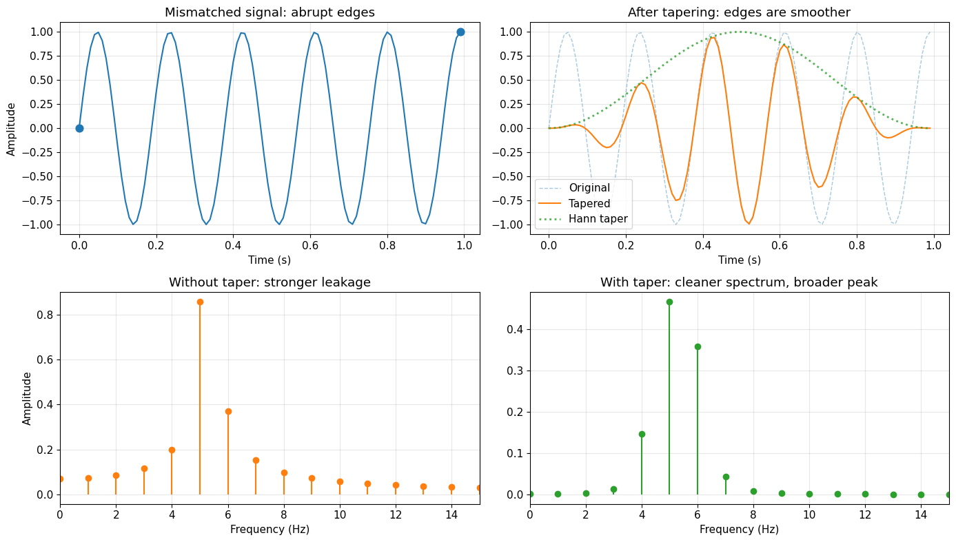
What changed?
- The taper reduces leakage into distant frequencies.
- The main peak becomes cleaner, but also slightly broader.

1.8 Tapering in Filtering: Edge Effects and Ringing¶

Filtering finite time series can create edge artifacts. These artifacts often look like oscillations near the start or end of the record, and are commonly called ringing.

To see this clearly, it helps to use an exaggerated example.

We will start with a clean 5 Hz sine wave, then deliberately create a sharp discontinuity at the boundaries. After that, we apply a narrow bandpass filter centered near 5 Hz.

If we do this without tapering, the filter reacts strongly to the sharp edge. If we taper first, the result is much cleaner.

# Stronger ringing demo: sharp edge + narrow bandpass filter
t_filt = np.arange(0, 2.0, 1/sampling_rate)

# Clean signal of interest
x_clean_filt = np.sin(2 * np.pi * 5 * t_filt)

# Create an exaggerated edge discontinuity
x_edge_filt = x_clean_filt + 2.0
x_edge_filt[0] = -3.0
x_edge_filt[-1] = 3.0

# Tapered version
taper_filt = windows.tukey(len(x_edge_filt), alpha=0.3)
x_tapered_filt = x_edge_filt * taper_filt

# Narrow bandpass around 5 Hz
b, a = butter(8, [4.5, 5.5], btype='band', fs=sampling_rate)

# Filtered outputs
x_filt_notaper = filtfilt(b, a, x_edge_filt)
x_filt_withtaper = filtfilt(b, a, x_tapered_filt)

fig, axes = plt.subplots(3, 2, figsize=(13, 9), sharey='row')

# Inputs
axes[0, 0].plot(t_filt, x_edge_filt)
axes[0, 0].set_title("Input without taper")
axes[0, 0].set_ylabel("Amplitude")
axes[0, 0].grid(True, alpha=0.3)

axes[0, 1].plot(t_filt, x_tapered_filt)
axes[0, 1].set_title("Input with taper")
axes[0, 1].grid(True, alpha=0.3)

# Full filtered outputs
axes[1, 0].plot(t_filt, x_filt_notaper)
axes[1, 0].set_title("Filtered without taper")
axes[1, 0].set_ylabel("Amplitude")
axes[1, 0].grid(True, alpha=0.3)

axes[1, 1].plot(t_filt, x_filt_withtaper)
axes[1, 1].set_title("Filtered with taper")
axes[1, 1].grid(True, alpha=0.3)

# Left-edge zoom
axes[2, 0].plot(t_filt, x_filt_notaper)
axes[2, 0].set_xlim(0, 0.4)
axes[2, 0].set_title("Left-edge zoom: no taper")
axes[2, 0].set_xlabel("Time (s)")
axes[2, 0].set_ylabel("Amplitude")
axes[2, 0].grid(True, alpha=0.3)

axes[2, 1].plot(t_filt, x_filt_withtaper)
axes[2, 1].set_xlim(0, 0.4)
axes[2, 1].set_title("Left-edge zoom: with taper")
axes[2, 1].set_xlabel("Time (s)")
axes[2, 1].grid(True, alpha=0.3)

plt.tight_layout()
plt.show()

left_notaper = np.max(np.abs(x_filt_notaper[:40]))
left_taper = np.max(np.abs(x_filt_withtaper[:40]))

print("What to notice:")
print("- Without tapering, the filter creates large oscillations near the edge.")
print("- With tapering, the edge artifact is much smaller.")
if left_taper > 0:
    print(f"- Near the left edge, the artifact is about {left_notaper/left_taper:.1f}x larger without tapering.")

print("\nKey idea:")
print("The ringing is not a physical signal. It is created by filtering a sharp boundary.")

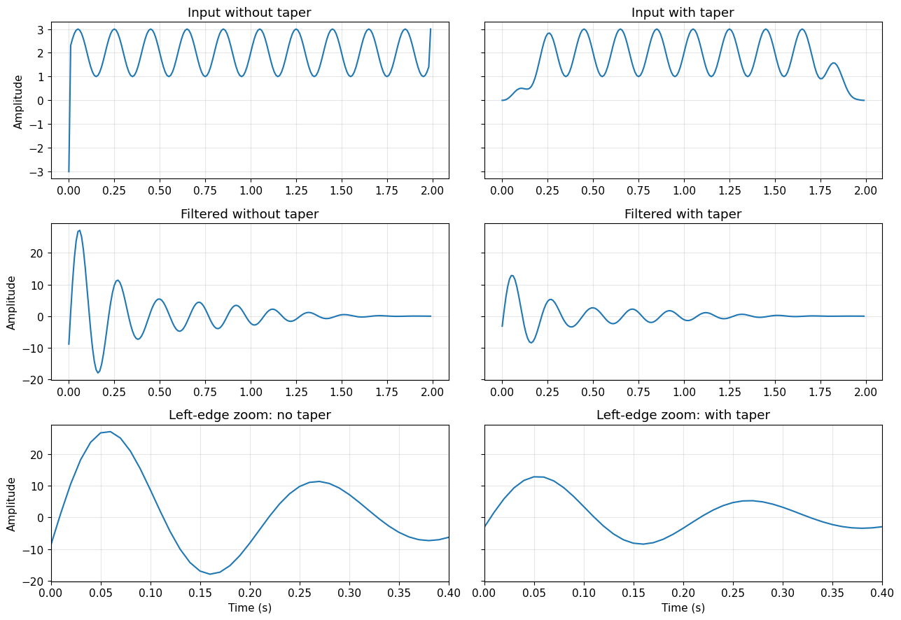
What to notice:
- Without tapering, the filter creates large oscillations near the edge.
- With tapering, the edge artifact is much smaller.
- Near the left edge, the artifact is about 2.1x larger without tapering.

Key idea:
The ringing is not a physical signal. It is created by filtering a sharp boundary.

1.9 Tapering and Differentiation/Integration: Boundary Artifacts Amplified¶

Differentiation and integration operations are particularly sensitive to discontinuities at time series boundaries. Remember:

Differentiation amplifies high frequencies → Makes edge discontinuities WORSE
Integration amplifies low frequencies → Can create long-period drift from DC offsets at edges

When we perform these operations in seismology (e.g., converting acceleration to velocity to displacement), boundary artifacts get amplified and propagate into our data. Tapering removes these edge discontinuities BEFORE the operations.

# Create toy signal with edge discontinuity
t_toy = np.arange(0, 2.0, 1/sampling_rate)
# Signal with LARGE low-frequency + high DC offset = HUGE edge discontinuity
# Differentiation will AMPLIFY this massively!
x_toy = 3.0*np.sin(2*np.pi*0.7*t_toy) + np.sin(2*np.pi*3*t_toy) + 2.5

# Differentiate in frequency domain (multiply by iω)
X_toy = np.fft.fft(x_toy)
freqs_toy = np.fft.fftfreq(len(x_toy), 1/sampling_rate)
omega = 2*np.pi*freqs_toy

# WITHOUT tapering
dx_notaper = np.real(np.fft.ifft(1j * omega * X_toy))

# WITH tapering
taper_toy = windows.hann(len(x_toy))
x_toy_tapered = x_toy * taper_toy
X_toy_tapered = np.fft.fft(x_toy_tapered)
dx_tapered = np.real(np.fft.ifft(1j * omega * X_toy_tapered))

# Plot comparison
fig, axes = plt.subplots(2, 2, figsize=(14, 10))

# Row 1: Original signals
axes[0,0].plot(t_toy, x_toy, 'k-', linewidth=1.5, label='Untapered')
axes[0,0].axhline(0, color='cyan', linestyle=':', linewidth=1)
axes[0,0].axvspan(0, 0.2, alpha=0.2, color='red')
axes[0,0].axvspan(1.8, 2.0, alpha=0.2, color='red')
axes[0,0].set_ylabel('Amplitude', fontsize=11)
axes[0,0].set_title('Original Signal (Large 0.7 Hz + 3 Hz + DC = 2.5)', fontsize=11, fontweight='bold')
axes[0,0].legend()
axes[0,0].grid(True, alpha=0.3)
axes[0,0].set_xlim([0, 2])
axes[0,0].set_ylim([-1, 6])

axes[0,1].plot(t_toy, x_toy_tapered, 'g-', linewidth=1.5, label='Tapered')
axes[0,1].axhline(0, color='gray', linestyle=':', linewidth=1)
axes[0,1].set_ylabel('Amplitude', fontsize=11)
axes[0,1].set_title('Tapered Signal (smooth edges)', fontsize=11, fontweight='bold')
axes[0,1].legend()
axes[0,1].grid(True, alpha=0.3)
axes[0,1].set_xlim([0, 2])
axes[0,1].set_ylim([-1, 6])

# Row 2: After differentiation
axes[1,0].plot(t_toy, dx_notaper, 'r-', linewidth=1.5)
axes[1,0].axhline(0, color='gray', linestyle=':', linewidth=1)
axes[1,0].axvspan(0, 0.4, alpha=0.3, color='red', label='EXTREME artifacts!')
axes[1,0].axvspan(1.6, 2.0, alpha=0.3, color='red')
axes[1,0].set_ylabel('Amplitude', fontsize=11)
axes[1,0].set_xlabel('Time (s)', fontsize=12)
axes[1,0].set_title('After Differentiation WITHOUT Taper: MASSIVE Artifacts!', fontsize=11, fontweight='bold', color='red')
axes[1,0].legend()
axes[1,0].grid(True, alpha=0.3)
axes[1,0].set_xlim([0, 2])
axes[1,0].set_ylim([-100, 100])

axes[1,1].plot(t_toy, dx_tapered, 'g-', linewidth=1.5)
axes[1,1].axhline(0, color='gray', linestyle=':', linewidth=1)
axes[1,1].set_ylabel('Amplitude', fontsize=11)
axes[1,1].set_xlabel('Time (s)', fontsize=12)
axes[1,1].set_title('After Differentiation WITH Taper: Clean Result', fontsize=11, fontweight='bold', color='green')
axes[1,1].grid(True, alpha=0.3)
axes[1,1].set_xlim([0, 2])
axes[1,1].set_ylim([-100, 100])

plt.tight_layout()
plt.show()

print("Maximum artifact magnitude WITHOUT tapering:")
print(f"  Near start: {np.max(np.abs(dx_notaper[:50])):.1f}")
print(f"  Near end: {np.max(np.abs(dx_notaper[-50:])):.1f}")
print(f"  Central region: {np.max(np.abs(dx_notaper[len(dx_notaper)//3:2*len(dx_notaper)//3])):.1f}")
print("\nMaximum magnitude WITH tapering:")
print(f"  Near start: {np.max(np.abs(dx_tapered[:50])):.1f}")
print(f"  Near end: {np.max(np.abs(dx_tapered[-50:])):.1f}")
print(f"  Central region: {np.max(np.abs(dx_tapered[len(dx_tapered)//3:2*len(dx_tapered)//3])):.1f}")
print(f"\n🚨 Edge artifacts are {np.max(np.abs(dx_notaper[:50]))/np.max(np.abs(dx_tapered[len(dx_tapered)//3:2*len(dx_tapered)//3])):.0f}× LARGER than the true signal!")
print("Without tapering, you can't even see the real signal - it's drowned in artifacts!")
print("\n⚠️  In seismology: Integration/differentiation WITHOUT tapering = GARBAGE DATA")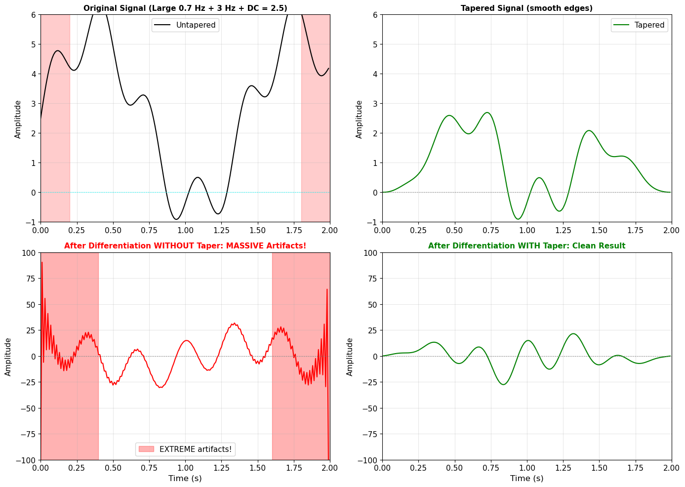

Maximum artifact magnitude WITHOUT tapering:
  Near start: 102.1
  Near end: 118.7
  Central region: 30.8

Maximum magnitude WITH tapering:
  Near start: 13.3
  Near end: 8.5
  Central region: 27.6

🚨 Edge artifacts are 4× LARGER than the true signal!
Without tapering, you can't even see the real signal - it's drowned in artifacts!

⚠️  In seismology: Integration/differentiation WITHOUT tapering = GARBAGE DATA

📌 Summary: Why Tapering Matters¶

The Core Problem:

The FFT assumes your time series is periodic (repeats infinitely)
Real data has finite duration with arbitrary start/end values
This creates an implicit discontinuity when the FFT “wraps” the signal
Result: Non-physical high-frequency energy (spectral leakage) and edge artifacts

When to Taper:

✅ Before computing spectra (always!)
✅ Before filtering (prevents edge ringing)
✅ Before differentiation/integration (prevents artifact amplification)
✅ When analyzing windows of continuous data
✅ Before cross-correlation (edge effects contaminate results)

Common Tapers in Seismology:

Hann (Hanning): Smooth, good general purpose (0 at edges)
Tukey (Tapered Cosine): Only tapers edges (α parameter controls taper width, e.g., 5-10%)
Cosine: Simple, symmetric taper
Multitaper: Advanced method for spectral estimation (covered in advanced courses)

The Trade-off:

Tapering reduces usable data at the edges
But it eliminates non-physical artifacts that would contaminate the entire analysis
In seismology: Better to lose edge data than to have artifacts contaminate everything

Remember: The artifacts you see WITHOUT tapering are NOT real—they’re mathematical artifacts from the FFT’s periodicity assumption. When in doubt, taper!

Summary: Key Concepts from Theory¶

Before moving to real data, let’s summarize what we’ve learned:

Concept	Time Domain	Frequency Domain
Pure sine	Single oscillation	Single peak at that frequency
Multiple frequencies	Complex waveform	Multiple peaks
Integration	Smooths signal, divides by $2\pi f$	Divides spectrum by $f$ (suppresses high freq)
Differentiation	Enhances rapid changes, multiplies by $2\pi f$	Multiplies spectrum by $f$ (enhances high freq)

Physical Meaning in Seismology:

Displacement = where the ground moved to
Velocity = how fast the ground moved
Acceleration = how rapidly the velocity changed (what you feel!)

2. Real Observations - Seismic Data Analysis¶

Now let’s apply everything we’ve learned to real earthquake recordings!

2.1 Seismic Data Access with ObsPy¶

ObsPy is the standard Python framework for seismology. It provides:

Access to global seismic data archives (IRIS, SCEDC, etc.)
Data processing tools (filtering, integration, etc.)
Format conversions and instrument response removal

We’ll download data from a real earthquake and apply Fourier analysis.

# Import ObsPy (install if needed in Colab)
try:
    import obspy
    from obspy.clients.fdsn import Client
    from obspy import UTCDateTime
except ImportError:
    !pip install obspy
    import obspy
    from obspy.clients.fdsn import Client
    from obspy import UTCDateTime

print(f"ObsPy version: {obspy.__version__}")
print("ObsPy loaded successfully!")

ObsPy version: 1.5.0
ObsPy loaded successfully!

2.2 Find and Download an Earthquake¶

Let’s search for a recent moderate earthquake and download seismic data.

# Connect to IRIS earthquake catalog
client = Client("IRIS")

# Search for earthquakes in a specific time window
t1 = UTCDateTime("2022-12-20")  # Start date
t2 = t1 + 86400  # One day later

# Get events M6+ (good signal-to-noise)
catalog = client.get_events(starttime=t1, endtime=t2, minmagnitude=6.0)

print(f"Found {len(catalog)} earthquake(s) with M ≥ 6.0")
print("\nEvent details:")

for i, event in enumerate(catalog):
    origin = event.origins[0]
    magnitude = event.magnitudes[0]
    
    print(f"\nEvent {i+1}:")
    print(f"  Time: {origin.time}")
    print(f"  Magnitude: {magnitude.mag} {magnitude.magnitude_type}")
    print(f"  Location: {origin.latitude:.2f}°N, {origin.longitude:.2f}°E")
    print(f"  Depth: {origin.depth/1000:.1f} km")

# Select the first (or largest) event
event = catalog[0]
origin = event.origins[0]
magnitude = event.magnitudes[0]

# Extract event parameters
t0 = origin.time
lat0 = origin.latitude
lon0 = origin.longitude
depth0 = origin.depth / 1000  # Convert to km
mag0 = magnitude.mag

print(f"\n{'='*50}")
print(f"Selected event: M{mag0:.1f} at {t0}")
print(f"{'='*50}")

Found 1 earthquake(s) with M ≥ 6.0

Event details:

Event 1:
  Time: 2022-12-20T10:34:24.770000Z
  Magnitude: 6.4 mw
  Location: 40.52°N, -124.42°E
  Depth: 17.9 km

==================================================
Selected event: M6.4 at 2022-12-20T10:34:24.770000Z
==================================================

2.3 Download Seismic Data from a Nearby Station¶

Now let’s find a station that recorded this earthquake and download the data.

Station components:

Z = Vertical
N = North-South horizontal
E = East-West horizontal

# Search for stations within ~400 km of earthquake
max_radius = 3.5  # degrees (roughly 350-400 km)

# Look for strong motion or broadband stations
# HN* = strong motion accelerometer
# HH* = broadband high-sample-rate
stations = client.get_stations(network="UO,UW", station="*", channel="HN*,HH*",
                                latitude=lat0, longitude=lon0,
                                maxradius=max_radius,
                                starttime=t0-1800, endtime=t0+7200,
                                level="channel")

print(f"Found {len(stations[0])} station(s)")
print(f"\nAvailable stations:")
for net in stations:
    for sta in net:
        print(f"  {net.code}.{sta.code} ({sta.latitude:.2f}°N, {sta.longitude:.2f}°E)")
        for chan in sta:
            print(f"    Channel: {chan.code}")

# Select a station (modify as needed based on what's available)
network = stations[0].code
station = stations[0][0].code

print(f"\n{'='*50}")
print(f"Selected station: {network}.{station}")
print(f"{'='*50}")

Found 39 station(s)

Available stations:
  UO.BASIN (42.18°N, -124.12°E)
    Channel: HNE
    Channel: HNN
    Channel: HNZ
  UO.BENT (42.96°N, -124.27°E)
    Channel: HNE
    Channel: HNN
    Channel: HNZ
  UO.CARP (42.23°N, -124.34°E)
    Channel: HNE
    Channel: HNN
    Channel: HNZ
  UO.CAVE (42.12°N, -123.57°E)
    Channel: HHE
    Channel: HHN
    Channel: HHZ
  UO.CHUCK (42.01°N, -124.20°E)
    Channel: HHE
    Channel: HHN
    Channel: HHZ
  UO.COQI (43.19°N, -124.18°E)
    Channel: HNE
    Channel: HNN
    Channel: HNZ
  UO.DAYS (42.97°N, -123.17°E)
    Channel: HNE
    Channel: HNN
    Channel: HNZ
  UO.DBO (43.12°N, -123.24°E)
    Channel: HHE
    Channel: HHN
    Channel: HHZ
  UO.DEAN (43.61°N, -123.98°E)
    Channel: HHE
    Channel: HHN
    Channel: HHZ
  UO.DFAZ (43.24°N, -122.11°E)
    Channel: HHE
    Channel: HHN
    Channel: HHZ
  UO.DING (42.86°N, -124.05°E)
    Channel: HHE
    Channel: HHN
    Channel: HHZ
  UO.DRAN (43.70°N, -123.35°E)
    Channel: HHE
    Channel: HHN
    Channel: HHZ
  UO.DUTCH (42.04°N, -122.89°E)
    Channel: HHE
    Channel: HHN
    Channel: HHZ
  UO.ETON (43.64°N, -123.58°E)
    Channel: HNE
    Channel: HNN
    Channel: HNZ
  UO.HBUG (42.64°N, -124.38°E)
    Channel: HHE
    Channel: HHN
    Channel: HHZ
  UO.HSO2 (43.52°N, -123.11°E)
    Channel: HHE
    Channel: HHN
    Channel: HHZ
  UO.IRYS (43.89°N, -123.26°E)
    Channel: HHE
    Channel: HHN
    Channel: HHZ
  UO.KBO (42.21°N, -124.23°E)
    Channel: HHE
    Channel: HHN
    Channel: HHZ
  UO.KEB (42.87°N, -124.33°E)
    Channel: HHE
    Channel: HHN
    Channel: HHZ
  UO.KING (42.69°N, -123.23°E)
    Channel: HHE
    Channel: HHN
    Channel: HHZ
  UO.LAIR (43.16°N, -123.93°E)
    Channel: HHE
    Channel: HHN
    Channel: HHZ
  UO.LAKE (43.58°N, -124.18°E)
    Channel: HNE
    Channel: HNN
    Channel: HNZ
  UO.LONE (43.36°N, -123.06°E)
    Channel: HHE
    Channel: HHN
    Channel: HHZ
  UO.LOST (42.02°N, -121.50°E)
    Channel: HNE
    Channel: HNN
    Channel: HNZ
  UO.MERL (42.50°N, -123.38°E)
    Channel: HNE
    Channel: HNN
    Channel: HNZ
  UO.OLBLU (43.51°N, -123.67°E)
    Channel: HHE
    Channel: HHN
    Channel: HHZ
  UO.RANT (42.03°N, -121.28°E)
    Channel: HHE
    Channel: HHN
    Channel: HHZ
  UO.REDMO (42.12°N, -124.30°E)
    Channel: HHE
    Channel: HHN
    Channel: HHZ
  UO.ROGE (42.70°N, -123.67°E)
    Channel: HHE
    Channel: HHN
    Channel: HHZ
  UO.ROXY (42.35°N, -122.79°E)
    Channel: HNE
    Channel: HNN
    Channel: HNZ
  UO.RUCH (42.22°N, -123.05°E)
    Channel: HNE
    Channel: HNN
    Channel: HNZ
  UO.SALT (42.49°N, -122.59°E)
    Channel: HHE
    Channel: HHN
    Channel: HHZ
  UO.SISQ (42.28°N, -123.63°E)
    Channel: HHE
    Channel: HHN
    Channel: HHZ
  UO.SNAKE (42.47°N, -124.16°E)
    Channel: HNE
    Channel: HNN
    Channel: HNZ
  UO.TBLE (42.93°N, -123.56°E)
    Channel: HHE
    Channel: HHN
    Channel: HHZ
  UO.VAUN (43.39°N, -123.89°E)
    Channel: HNE
    Channel: HNN
    Channel: HNZ
  UO.VINO (43.43°N, -123.42°E)
    Channel: HHE
    Channel: HHN
    Channel: HHZ
  UO.WOOD (42.22°N, -122.30°E)
    Channel: HHE
    Channel: HHN
    Channel: HHZ
  UO.WYLD (43.14°N, -123.43°E)
    Channel: HHE
    Channel: HHN
    Channel: HHZ
  UW.BAND (43.09°N, -124.41°E)
    Channel: HNE
    Channel: HNN
    Channel: HNZ
  UW.BBO (42.89°N, -122.68°E)
    Channel: HHE
    Channel: HHN
    Channel: HHZ
  UW.BROK (42.08°N, -124.29°E)
    Channel: HNE
    Channel: HNN
    Channel: HNZ
  UW.CABL (42.84°N, -124.56°E)
    Channel: HNE
    Channel: HNN
    Channel: HNZ
  UW.COOS (43.40°N, -124.25°E)
    Channel: HNE
    Channel: HNN
    Channel: HNZ
  UW.FLRE (43.99°N, -124.11°E)
    Channel: HNE
    Channel: HNN
    Channel: HNZ
  UW.HOG (42.24°N, -121.71°E)
    Channel: HNE
    Channel: HNN
    Channel: HNZ
  UW.JEDS (43.75°N, -124.05°E)
    Channel: HHE
    Channel: HHN
    Channel: HHZ
  UW.KFAL (42.26°N, -121.79°E)
    Channel: HNE
    Channel: HNN
    Channel: HNZ
  UW.REED (43.70°N, -124.11°E)
    Channel: HNE
    Channel: HNN
    Channel: HNZ
  UW.RNO2 (43.91°N, -123.74°E)
    Channel: HNE
    Channel: HNN
    Channel: HNZ
  UW.TREE (42.73°N, -120.89°E)
    Channel: HHE
    Channel: HHN
    Channel: HHZ
  UW.WEDR (42.44°N, -124.41°E)
    Channel: HNE
    Channel: HNN
    Channel: HNZ

==================================================
Selected station: UO.BASIN
==================================================

# Download waveform data (vertical component)
# Time window: a bit before earthquake to ~10 minutes after
starttime = t0 - 200
endtime = t0 + 600

# Try to get HNZ (strong motion) first, fall back to HHZ (broadband)
try:
    stream = client.get_waveforms(network, station, "*", "HNZ",
                                   starttime, endtime,
                                   attach_response=True)
    channel_type = "HN (Strong Motion Accelerometer)"
except:
    stream = client.get_waveforms(network, station, "*", "HHZ",
                                   starttime, endtime,
                                   attach_response=True)
    channel_type = "HH (Broadband)"

print(f"Downloaded {len(stream)} trace(s)")
print(f"Channel type: {channel_type}")
print(f"\nStream info:")
print(stream)

# Get the trace
tr = stream[0]

print(f"\nTrace statistics:")
print(f"  Sampling rate: {tr.stats.sampling_rate} Hz")
print(f"  Number of samples: {tr.stats.npts}")
print(f"  Duration: {tr.stats.npts / tr.stats.sampling_rate:.1f} seconds")
print(f"  Start time: {tr.stats.starttime}")
print(f"  End time: {tr.stats.endtime}")

Downloaded 1 trace(s)
Channel type: HN (Strong Motion Accelerometer)

Stream info:
1 Trace(s) in Stream:
UO.BASIN..HNZ | 2022-12-20T10:31:04.770000Z - 2022-12-20T10:44:24.770000Z | 200.0 Hz, 160001 samples

Trace statistics:
  Sampling rate: 200.0 Hz
  Number of samples: 160001
  Duration: 800.0 seconds
  Start time: 2022-12-20T10:31:04.770000Z
  End time: 2022-12-20T10:44:24.770000Z

2.4 Instrument Response and Ground Motion Units¶

Problem: Seismometers don’t directly measure ground motion - they measure voltage!

The instrument response describes how the seismometer converts ground motion → voltage.

Common recording units:

Counts: Raw digital numbers from the instrument
Velocity: What broadband seismometers naturally measure (m/s)
Acceleration: What strong motion sensors measure (m/s²)
Displacement: Integrated from velocity or acceleration (m)

We need to remove the instrument response to get true ground motion.

# Remove instrument response to get acceleration
tr_acc = tr.copy()
tr_acc.remove_response(output="ACC")  # Output in m/s²

# Plot raw waveform
fig, ax = plt.subplots(figsize=(14, 5))

time_relative = tr_acc.times(reftime=t0)  # Time relative to earthquake origin
ax.plot(time_relative, tr_acc.data, 'b-', linewidth=0.8)
ax.axvline(0, color='red', linestyle='--', linewidth=2, label='Earthquake origin time')
ax.set_xlabel('Time after earthquake origin (s)', fontsize=12)
ax.set_ylabel('Acceleration (m/s²)', fontsize=12)
ax.set_title(f'Seismogram: {network}.{station}.{tr.stats.channel} - M{mag0:.1f} Earthquake', 
             fontsize=13, fontweight='bold')
ax.legend()
ax.grid(True, alpha=0.3)

plt.tight_layout()
plt.show()

print(f"Peak ground acceleration: {np.max(np.abs(tr_acc.data)):.4f} m/s²")
print(f"That's {np.max(np.abs(tr_acc.data))/9.81:.3f} times Earth's gravity!")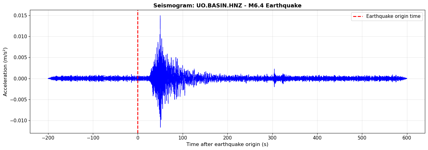

Peak ground acceleration: 0.0150 m/s²
That's 0.002 times Earth's gravity!

2.5 Integration: Acceleration → Velocity → Displacement¶

Now let’s apply what we learned in Part 1 to real data!

# Get the data arrays
acc_data = tr_acc.data
dt = tr_acc.stats.delta  # Time step

# Integrate to get velocity
vel_data = cumulative_trapezoid(acc_data, dx=dt, initial=0)

# Integrate again to get displacement
disp_data = cumulative_trapezoid(vel_data, dx=dt, initial=0)

# Plot all three
fig, axes = plt.subplots(3, 1, figsize=(14, 10), sharex=True)

time_rel = tr_acc.times(reftime=t0)

# Acceleration
axes[0].plot(time_rel, acc_data, 'b-', linewidth=0.8)
axes[0].axvline(0, color='red', linestyle='--', alpha=0.5)
axes[0].set_ylabel('Acceleration\n(m/s²)', fontsize=11, fontweight='bold')
axes[0].set_title(f'Real Seismogram: {network}.{station} - Acceleration → Velocity → Displacement', 
                  fontsize=13, fontweight='bold')
axes[0].grid(True, alpha=0.3)

# Velocity
axes[1].plot(time_rel, vel_data, 'g-', linewidth=0.8)
axes[1].axvline(0, color='red', linestyle='--', alpha=0.5)
axes[1].set_ylabel('Velocity\n(m/s)', fontsize=11, fontweight='bold')
axes[1].grid(True, alpha=0.3)

# Displacement
axes[2].plot(time_rel, disp_data, 'r-', linewidth=0.8)
axes[2].axvline(0, color='red', linestyle='--', alpha=0.5, label='Origin time')
axes[2].set_ylabel('Displacement\n(m)', fontsize=11, fontweight='bold')
axes[2].set_xlabel('Time after earthquake origin (s)', fontsize=12)
axes[2].legend()
axes[2].grid(True, alpha=0.3)

plt.tight_layout()
plt.show()

print("Observations (compare to toy problem):")
print("1. Integration smooths the signal (removes high frequencies)")
print("2. Displacement shows longer-period motion")
print("3. Peak acceleration ≠ peak displacement!")
print(f"\n   Peak acceleration: {np.max(np.abs(acc_data)):.4f} m/s²")
print(f"   Peak velocity: {np.max(np.abs(vel_data)):.4f} m/s")
print(f"   Peak displacement: {np.max(np.abs(disp_data)):.4f} m")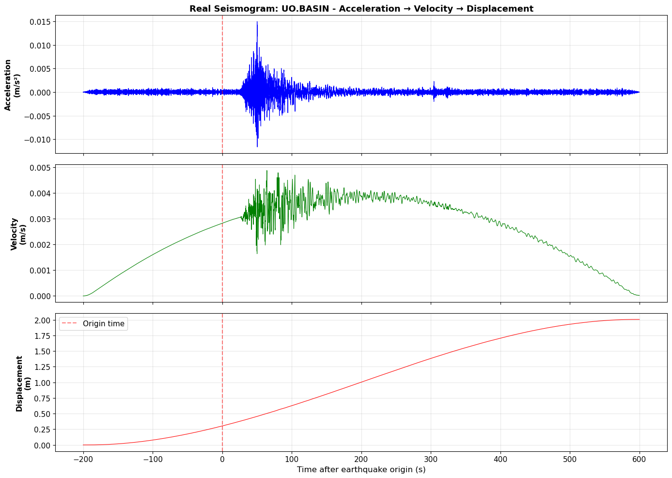

Observations (compare to toy problem):
1. Integration smooths the signal (removes high frequencies)
2. Displacement shows longer-period motion
3. Peak acceleration ≠ peak displacement!

   Peak acceleration: 0.0150 m/s²
   Peak velocity: 0.0049 m/s
   Peak displacement: 2.0051 m

2.7 Fourier Analysis of Real Seismograms¶

Now let’s look at the spectral content - what frequencies are in this earthquake signal?

# Compute Fourier transforms
N_real = len(acc_data)
Acc_fft = np.abs(fft(acc_data)[:N_real//2])
Vel_fft = np.abs(fft(vel_data)[:N_real//2])
Disp_fft = np.abs(fft(disp_data)[:N_real//2])

# Frequency axis
freqs_real = fftfreq(N_real, dt)[:N_real//2]

# Plot spectra
fig, (ax1, ax2) = plt.subplots(1, 2, figsize=(14, 5))

# Linear scale
ax1.plot(freqs_real, Acc_fft, 'b-', linewidth=1.5, label='Acceleration', alpha=0.7)
ax1.plot(freqs_real, Vel_fft, 'g-', linewidth=1.5, label='Velocity', alpha=0.7)
ax1.plot(freqs_real, Disp_fft, 'r-', linewidth=1.5, label='Displacement', alpha=0.7)
ax1.set_xlabel('Frequency (Hz)', fontsize=12)
ax1.set_ylabel('Amplitude Spectrum', fontsize=12)
ax1.set_title('Frequency Spectra - Linear Scale', fontsize=13, fontweight='bold')
ax1.legend(fontsize=11)
ax1.grid(True, alpha=0.3)
ax1.set_xlim([0, 20])
ax1.set_ylim([0, 1000])

# Log-log scale (easier to see pattern)
ax2.loglog(freqs_real[1:], Acc_fft[1:], 'b-', linewidth=2, label='Acceleration', alpha=0.7)
ax2.loglog(freqs_real[1:], Vel_fft[1:], 'g-', linewidth=2, label='Velocity', alpha=0.7)
ax2.loglog(freqs_real[1:], Disp_fft[1:], 'r-', linewidth=2, label='Displacement', alpha=0.7)
ax2.set_xlabel('Frequency (Hz)', fontsize=12)
ax2.set_ylabel('Amplitude Spectrum (log)', fontsize=12)
ax2.set_title('Frequency Spectra - Log-Log Scale', fontsize=13, fontweight='bold')
ax2.legend(fontsize=11)
ax2.grid(True, alpha=0.3, which='both')
ax2.set_xlim([0.1, 50])

plt.tight_layout()
plt.show()

# Find dominant frequency
peak_idx = np.argmax(Acc_fft[freqs_real > 0.1])  # Ignore DC component
peak_freq = freqs_real[freqs_real > 0.1][peak_idx]

print(f"Dominant frequency: {peak_freq:.2f} Hz (period = {1/peak_freq:.2f} s)")
print("\nObservations:")
print("1. Earthquake energy concentrated in 0.5-10 Hz range")
print("2. Spectra show characteristic 1/f relationship between acc, vel, disp")
print("3. Low frequencies (< 1 Hz) dominate displacement")
print("4. High frequencies (> 5 Hz) dominate acceleration")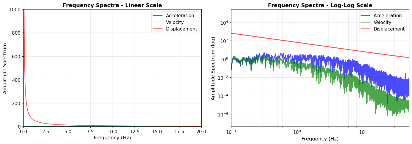

Dominant frequency: 0.31 Hz (period = 3.17 s)

Observations:
1. Earthquake energy concentrated in 0.5-10 Hz range
2. Spectra show characteristic 1/f relationship between acc, vel, disp
3. Low frequencies (< 1 Hz) dominate displacement
4. High frequencies (> 5 Hz) dominate acceleration

2.6 Applying Tapering to Real Seismic Data¶

Now let’s apply the tapering concepts from Part 1 to our real earthquake data. Recall from the toy problems that tapering is crucial for:

Computing spectra (prevents spectral leakage)
Filtering (prevents edge ringing)
Differentiating/integrating (prevents artifact amplification)

We’ll extract a window from our acceleration data and demonstrate all three applications. Real seismic records rarely start and end at zero, so edge artifacts can severely contaminate your analysis without proper tapering.

# Extract a 30-second window from the real acceleration data
# This simulates analyzing a portion of a seismogram
start_idx = 5000  # Start somewhere in the middle
window_length = int(30 * tr_acc.stats.sampling_rate)  # 30 seconds
data_window = tr_acc.data[start_idx:start_idx + window_length]
time_window = np.arange(len(data_window)) / tr_acc.stats.sampling_rate

# Compute spectra WITHOUT and WITH tapering
# WITHOUT taper
fft_notaper = np.fft.rfft(data_window)
freqs_real = np.fft.rfftfreq(len(data_window), 1/tr_acc.stats.sampling_rate)
spectrum_notaper = np.abs(fft_notaper)

# WITH taper (5% Tukey taper - common in seismology)
taper_real = windows.tukey(len(data_window), alpha=0.05)
data_tapered = data_window * taper_real
fft_tapered = np.fft.rfft(data_tapered)
spectrum_tapered = np.abs(fft_tapered)

# Also filter this window to show filtering artifacts
b, a = butter(4, [0.1, 10], btype='band', fs=tr_acc.stats.sampling_rate)
data_filt_notaper = filtfilt(b, a, data_window)
data_filt_withtaper = filtfilt(b, a, data_tapered)

# Create comparison plot
fig = plt.figure(figsize=(16, 12))
gs = fig.add_gridspec(3, 2, hspace=0.3, wspace=0.3)

# Row 1: Time domain - original window
ax1 = fig.add_subplot(gs[0, 0])
ax1.plot(time_window, data_window, 'k-', linewidth=0.8)
ax1.axhline(0, color='gray', linestyle=':', linewidth=1)
ax1.axvspan(0, 1.5, alpha=0.2, color='red', label='Edge regions')
ax1.axvspan(28.5, 30, alpha=0.2, color='red')
ax1.set_ylabel('Acceleration (m/s²)', fontsize=11)
ax1.set_title('30-Second Window of Real Seismic Data (Untapered)', fontsize=11, fontweight='bold')
ax1.legend()
ax1.grid(True, alpha=0.3)
ax1.set_xlim([0, 30])

ax2 = fig.add_subplot(gs[0, 1])
ax2.plot(time_window, data_tapered, 'g-', linewidth=0.8)
ax2.axhline(0, color='cyan', linestyle=':', linewidth=1)
ax2.set_ylabel('Acceleration (m/s²)', fontsize=11)
ax2.set_title('Same Window WITH 5% Tukey Taper (Smooth Edges)', fontsize=11, fontweight='bold')
ax2.grid(True, alpha=0.3)
ax2.set_xlim([0, 30])

# Row 2: Frequency domain - spectra
ax3 = fig.add_subplot(gs[1, 0])
ax3.loglog(freqs_real[1:], spectrum_notaper[1:], 'b-', linewidth=1.5, alpha=0.7, label='Without taper')
ax3.set_ylabel('Amplitude', fontsize=11)
ax3.set_xlabel('Frequency (Hz)', fontsize=12)
ax3.set_title('Spectrum WITHOUT Tapering (Spectral Leakage)', fontsize=11, fontweight='bold')
ax3.legend()
ax3.grid(True, alpha=0.3, which='both')
ax3.set_xlim([0.01, 50])

ax4 = fig.add_subplot(gs[1, 1])
ax4.loglog(freqs_real[1:], spectrum_tapered[1:], 'g-', linewidth=1.5, alpha=0.7, label='With taper')
ax4.set_ylabel('Amplitude', fontsize=11)
ax4.set_xlabel('Frequency (Hz)', fontsize=12)
ax4.set_title('Spectrum WITH Tapering (Cleaner)', fontsize=11, fontweight='bold')
ax4.legend()
ax4.grid(True, alpha=0.3, which='both')
ax4.set_xlim([0.01, 50])

# Row 3: Filtered data comparison
ax5 = fig.add_subplot(gs[2, 0])
ax5.plot(time_window, data_filt_notaper, 'r-', linewidth=0.8)
ax5.axhline(0, color='gray', linestyle=':', linewidth=1)
ax5.axvspan(0, 2, alpha=0.3, color='red', label='Edge artifacts')
ax5.axvspan(28, 30, alpha=0.3, color='red')
ax5.set_ylabel('Acceleration (m/s²)', fontsize=11)
ax5.set_xlabel('Time (s)', fontsize=12)
ax5.set_title('Bandpass Filtered (0.1-10 Hz) WITHOUT Taper: Edge Ringing', fontsize=11, fontweight='bold', color='red')
ax5.legend()
ax5.grid(True, alpha=0.3)
ax5.set_xlim([0, 30])

ax6 = fig.add_subplot(gs[2, 1])
ax6.plot(time_window, data_filt_withtaper, 'g-', linewidth=0.8)
ax6.axhline(0, color='gray', linestyle=':', linewidth=1)
ax6.set_ylabel('Acceleration (m/s²)', fontsize=11)
ax6.set_xlabel('Time (s)', fontsize=12)
ax6.set_title('Bandpass Filtered (0.1-10 Hz) WITH Taper: Clean Edges', fontsize=11, fontweight='bold', color='green')
ax6.grid(True, alpha=0.3)
ax6.set_xlim([0, 30])

plt.show()

print("Real seismic data analysis:")
print(f"  Original window: {len(data_window)} samples ({len(data_window)/tr_acc.stats.sampling_rate:.1f} seconds)")
print(f"  Sampling rate: {tr_acc.stats.sampling_rate} Hz")
print(f"  Start value: {data_window[0]:.6e} m/s²")
print(f"  End value: {data_window[-1]:.6e} m/s²")
print(f"  → Discontinuity: {abs(data_window[-1] - data_window[0]):.6e} m/s²")
print("\n✅ Best practice: ALWAYS taper before:")
print("   - Computing spectra")
print("   - Filtering")
print("   - Differentiating/integrating")
print("   - Cross-correlating")
print("\n⚠️  Exception: When analyzing the full continuous record with proper DC removal.")
print("\n💡 Notice: Same tapering principles from toy problems apply perfectly to real data!")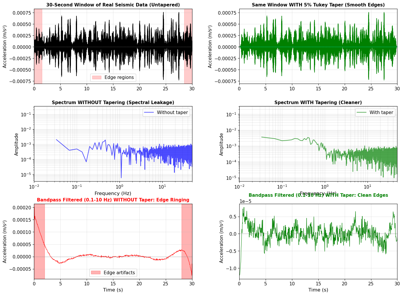

Real seismic data analysis:
  Original window: 6000 samples (30.0 seconds)
  Sampling rate: 200.0 Hz
  Start value: -2.186170e-04 m/s²
  End value: 6.388503e-05 m/s²
  → Discontinuity: 2.825020e-04 m/s²

✅ Best practice: ALWAYS taper before:
   - Computing spectra
   - Filtering
   - Differentiating/integrating
   - Cross-correlating

⚠️  Exception: When analyzing the full continuous record with proper DC removal.

💡 Notice: Same tapering principles from toy problems apply perfectly to real data!

Summary: Theory Meets Observation¶

We started with toy problems using simple sinusoids to understand:

Fourier transform decomposes signals into frequencies
Time domain ↔ Frequency domain are equivalent views
Integration divides spectrum by frequency (suppresses high freq)
Differentiation multiplies spectrum by frequency (enhances high freq)

Then we applied these concepts to real seismic data:

Downloaded earthquake recordings from IRIS
Removed instrument response to get ground motion
Integrated acceleration → velocity → displacement
Analyzed spectral content with Fourier transforms

Key Takeaways:

Same physics in toy problems and real earthquakes!
Frequency analysis reveals what simple time-domain inspection cannot
Choice of ground motion unit (acc/vel/disp) depends on application:
- Engineering (building response) → Acceleration
- Long-period seismology (Earth structure) → Displacement/Velocity
- Magnitude determination → Often velocity or displacement

Next Steps¶

In future notebooks, we’ll use these Fourier analysis skills for:

Filtering: Isolating specific frequency bands (body waves vs surface waves)
Spectrograms: Time-frequency analysis of dispersive waves
Transfer functions: Relating input to output through Earth’s structure

The Fourier transform is your most important tool in seismology - master it!